Part 2: Using the icepyx python library to access ICESat-2 data#
Tutorial Overview#
This tutorial is designed for the “Cloud Computing and Open-Source Scientific Software for Cryosphere Communities” Learning Workshop at the 2023 AGU Fall Meeting.
This notebook demonstrates how to search for, access, and analyse and plot a cloud-hosted ICESat-2 dataset using the icepyx package.
icepyx is a community and software library for searching, downloading, and reading ICESat-2 data. While opening data should be straightforward, there are some oddities in navigating the highly nested organization and hundreds of variables of the ICESat-2 data. icepyx provides tools to help with those oddities.
icepyx was started and initially developed by Jessica Scheick to provide easy programmatic access to ICESat-2 data (before earthaccess existed!) and facilitate collaborative development around ICESat-2 data products, including training, skill building, and support around practicing open science and contributing to open-source software. Thanks to contributions from countless community members, icepyx can (for ICESat-2 data):
search for available data granules (data files)
order and download data or access it directly in the cloud
order a subset of data: clipped in space, time, containing fewer variables, or a few other options provided by NSIDC
search through the available ICESat-2 data variables
read ICESat-2 data into xarray DataArrays, including merging data from multiple files
Under the hood, icepyx relies on earthaccess to help handle authentication, especially for obtaining S3 tokens to access ICESat-2 data in the cloud. All this happens without the user needing to take any action other than supplying their Earthdata Login credentials using one of the methods described in the earthaccess tutorial.
In this tutorial we will look at the ATL08 Land and Vegetation Height product.
Learning Objectives#
In this tutorial you will learn:
how to use
icepyxto search for ICESat-2 data using spatial and temporal filters;how to open and combine data multiple HDF5 groups into an
xarray.Datasetusingicepyx.Read;how to begin your analysis, including selecting strong/weak beams and plotting.
Prerequisites#
The workflow described in this tutorial forms the initial steps of an Analysis in Place workflow that would be run on a AWS cloud compute resource. You will need:
a JupyterHub, such as CryoHub, or AWS EC2 instance in the us-west-2 region.
a NASA Earthdata Login. If you need to register for an Earthdata Login see the Getting an Earthdata Login section of the ICESat-2 Hackweek 2023 Jupyter Book.
A
.netrcfile, that contains your Earthdata Login credentials, in your home directory. See Configure Programmatic Access to NASA Servers to create a.netrcfile.
Credits#
This notebook is based on an icepyx Tutorial originally created by Rachel Wegener, Univ. Maryland and updated by Amy Steiker, NSIDC, and Jessica Scheick, Univ. of New Hampshire. It was updated in May 2024 to utilize (at a minimum) v1.0.0 of icepyx.
Using icepyx to search and access ICESat-2 data#
We won’t dive into using icepyx to search for and download data in this tutorial, since we already discussed how to do that with earthaccess. The code to search and download is still provided below for the curious reader. The icepyx documentation shows more detail about different search parameters and how to inspect the results of a query.
import icepyx as ipx


import json
import math
import warnings

import numpy as np
import matplotlib.pyplot as plt
from matplotlib.colors import ListedColormap

from shapely.geometry import shape, GeometryCollection
%matplotlib inline
We’ll search for ATL08 tracks that intersect with the La Primavera Biosphere Reserve, Jalisco, Mexico, located west of Guadalajara.
# Open a geojson of our area of interest
with open("./bosque_primavera.json") as f:
    features = json.load(f)["features"]

bosque = GeometryCollection([shape(feature["geometry"]).buffer(0) for feature in features])
bosque

# Use our search parameters to setup a search Query
short_name = 'ATL08'
spatial_extent = list(bosque.bounds)
date_range = ['2019-05-04','2019-05-04']
region = ipx.Query(short_name, spatial_extent, date_range)
# Display if any data files, or granules, matched our search
region.avail_granules(ids=True)
[['ATL08_20190504124152_05540301_006_02.h5']]
# We can also get the S3 urls
print(region.avail_granules(ids=True, cloud=True))
s3urls = region.avail_granules(ids=True, cloud=True)[1]
[['ATL08_20190504124152_05540301_006_02.h5'], ['s3://nsidc-cumulus-prod-protected/ATLAS/ATL08/006/2019/05/04/ATL08_20190504124152_05540301_006_02.h5']]
# Download the granules to a into a folder called 'bosque_primavera_ATL08'
region.download_granules('./bosque_primavera_ATL08')
Total number of data order requests is  1  for  1  granules.
Data request  1  of  1  is submitting to NSIDC
order ID:  5000005555328
Initial status of your order request at NSIDC is:  processing
Your order status is still  processing  at NSIDC. Please continue waiting... this may take a few moments.
Your order is: complete
Beginning download of zipped output...
Data request 5000005555328 of  1  order(s) is downloaded.
Download complete
Reading a file with icepyx#
To read a file with icepyx there are several steps:
Create a
Readobject. This sets up an initial connection to your file(s) and validates the metadata.Tell the
Readobject what variables you would like to readLoad your data!
Create a Read object#
Here we are creating a read object to set up an initial connection to your file(s).
# access the file you've downloaded
reader = ipx.Read('./bosque_primavera_ATL08')
# access the file on the cloud (see "When to Cloud", below)
# reader = ipx.Read(s3urls)
reader
<icepyx.core.read.Read at 0x7f0fffdbcd90>
Select your variables#
To view the variables contained in your dataset you can call .vars on your data reader.
reader.vars.avail()
['ancillary_data/atlas_sdp_gps_epoch',
 'ancillary_data/control',
 'ancillary_data/data_end_utc',
 'ancillary_data/data_start_utc',
 'ancillary_data/end_cycle',
 'ancillary_data/end_delta_time',
 'ancillary_data/end_geoseg',
 'ancillary_data/end_gpssow',
 'ancillary_data/end_gpsweek',
 'ancillary_data/end_orbit',
 'ancillary_data/end_region',
 'ancillary_data/end_rgt',
 'ancillary_data/granule_end_utc',
 'ancillary_data/granule_start_utc',
 'ancillary_data/land/atl08_region',
 'ancillary_data/land/bin_size_h',
 'ancillary_data/land/bin_size_n',
 'ancillary_data/land/bright_thresh',
 'ancillary_data/land/ca_class',
 'ancillary_data/land/can_noise_thresh',
 'ancillary_data/land/can_stat_thresh',
 'ancillary_data/land/canopy20m_thresh',
 'ancillary_data/land/canopy_flag_switch',
 'ancillary_data/land/canopy_seg',
 'ancillary_data/land/class_thresh',
 'ancillary_data/land/cloud_filter_switch',
 'ancillary_data/land/del_amp',
 'ancillary_data/land/del_mu',
 'ancillary_data/land/del_sigma',
 'ancillary_data/land/dem_filter_switch',
 'ancillary_data/land/dem_removal_percent_limit',
 'ancillary_data/land/dragann_switch',
 'ancillary_data/land/dseg',
 'ancillary_data/land/dseg_buf',
 'ancillary_data/land/fnlgnd_filter_switch',
 'ancillary_data/land/gnd_stat_thresh',
 'ancillary_data/land/gthresh_factor',
 'ancillary_data/land/h_canopy_perc',
 'ancillary_data/land/iter_gnd',
 'ancillary_data/land/iter_max',
 'ancillary_data/land/lseg',
 'ancillary_data/land/lseg_buf',
 'ancillary_data/land/lw_filt_bnd',
 'ancillary_data/land/lw_gnd_bnd',
 'ancillary_data/land/lw_toc_bnd',
 'ancillary_data/land/lw_toc_cut',
 'ancillary_data/land/max_atl03files',
 'ancillary_data/land/max_atl09files',
 'ancillary_data/land/max_peaks',
 'ancillary_data/land/max_try',
 'ancillary_data/land/min_nphs',
 'ancillary_data/land/n_dec_mode',
 'ancillary_data/land/night_thresh',
 'ancillary_data/land/noise_class',
 'ancillary_data/land/outlier_filter_switch',
 'ancillary_data/land/p_static',
 'ancillary_data/land/ph_removal_percent_limit',
 'ancillary_data/land/proc_geoseg',
 'ancillary_data/land/psf',
 'ancillary_data/land/ref_dem_limit',
 'ancillary_data/land/ref_finalground_limit',
 'ancillary_data/land/relief_hbot',
 'ancillary_data/land/relief_htop',
 'ancillary_data/land/shp_param',
 'ancillary_data/land/sig_rsq_search',
 'ancillary_data/land/sseg',
 'ancillary_data/land/stat20m_thresh',
 'ancillary_data/land/stat_thresh',
 'ancillary_data/land/tc_thresh',
 'ancillary_data/land/te_class',
 'ancillary_data/land/terrain20m_thresh',
 'ancillary_data/land/toc_class',
 'ancillary_data/land/up_filt_bnd',
 'ancillary_data/land/up_gnd_bnd',
 'ancillary_data/land/up_toc_bnd',
 'ancillary_data/land/up_toc_cut',
 'ancillary_data/land/yapc_switch',
 'ancillary_data/qa_at_interval',
 'ancillary_data/release',
 'ancillary_data/start_cycle',
 'ancillary_data/start_delta_time',
 'ancillary_data/start_geoseg',
 'ancillary_data/start_gpssow',
 'ancillary_data/start_gpsweek',
 'ancillary_data/start_orbit',
 'ancillary_data/start_region',
 'ancillary_data/start_rgt',
 'ancillary_data/version',
 'ds_geosegments',
 'ds_metrics',
 'ds_surf_type',
 'gt3l/land_segments/asr',
 'gt3l/land_segments/atlas_pa',
 'gt3l/land_segments/beam_azimuth',
 'gt3l/land_segments/beam_coelev',
 'gt3l/land_segments/brightness_flag',
 'gt3l/land_segments/canopy/can_noise',
 'gt3l/land_segments/canopy/canopy_h_metrics',
 'gt3l/land_segments/canopy/canopy_h_metrics_abs',
 'gt3l/land_segments/canopy/canopy_openness',
 'gt3l/land_segments/canopy/canopy_rh_conf',
 'gt3l/land_segments/canopy/centroid_height',
 'gt3l/land_segments/canopy/h_canopy',
 'gt3l/land_segments/canopy/h_canopy_20m',
 'gt3l/land_segments/canopy/h_canopy_abs',
 'gt3l/land_segments/canopy/h_canopy_quad',
 'gt3l/land_segments/canopy/h_canopy_uncertainty',
 'gt3l/land_segments/canopy/h_dif_canopy',
 'gt3l/land_segments/canopy/h_max_canopy',
 'gt3l/land_segments/canopy/h_max_canopy_abs',
 'gt3l/land_segments/canopy/h_mean_canopy',
 'gt3l/land_segments/canopy/h_mean_canopy_abs',
 'gt3l/land_segments/canopy/h_median_canopy',
 'gt3l/land_segments/canopy/h_median_canopy_abs',
 'gt3l/land_segments/canopy/h_min_canopy',
 'gt3l/land_segments/canopy/h_min_canopy_abs',
 'gt3l/land_segments/canopy/n_ca_photons',
 'gt3l/land_segments/canopy/n_toc_photons',
 'gt3l/land_segments/canopy/photon_rate_can',
 'gt3l/land_segments/canopy/photon_rate_can_nr',
 'gt3l/land_segments/canopy/segment_cover',
 'gt3l/land_segments/canopy/subset_can_flag',
 'gt3l/land_segments/canopy/toc_roughness',
 'gt3l/land_segments/cloud_flag_atm',
 'gt3l/land_segments/cloud_fold_flag',
 'gt3l/land_segments/delta_time',
 'gt3l/land_segments/delta_time_beg',
 'gt3l/land_segments/delta_time_end',
 'gt3l/land_segments/dem_flag',
 'gt3l/land_segments/dem_h',
 'gt3l/land_segments/dem_removal_flag',
 'gt3l/land_segments/h_dif_ref',
 'gt3l/land_segments/last_seg_extend',
 'gt3l/land_segments/latitude',
 'gt3l/land_segments/latitude_20m',
 'gt3l/land_segments/layer_flag',
 'gt3l/land_segments/longitude',
 'gt3l/land_segments/longitude_20m',
 'gt3l/land_segments/msw_flag',
 'gt3l/land_segments/n_seg_ph',
 'gt3l/land_segments/night_flag',
 'gt3l/land_segments/ph_ndx_beg',
 'gt3l/land_segments/ph_removal_flag',
 'gt3l/land_segments/psf_flag',
 'gt3l/land_segments/rgt',
 'gt3l/land_segments/sat_flag',
 'gt3l/land_segments/segment_id_beg',
 'gt3l/land_segments/segment_id_end',
 'gt3l/land_segments/segment_landcover',
 'gt3l/land_segments/segment_snowcover',
 'gt3l/land_segments/segment_watermask',
 'gt3l/land_segments/sigma_across',
 'gt3l/land_segments/sigma_along',
 'gt3l/land_segments/sigma_atlas_land',
 'gt3l/land_segments/sigma_h',
 'gt3l/land_segments/sigma_topo',
 'gt3l/land_segments/snr',
 'gt3l/land_segments/solar_azimuth',
 'gt3l/land_segments/solar_elevation',
 'gt3l/land_segments/surf_type',
 'gt3l/land_segments/terrain/h_te_best_fit',
 'gt3l/land_segments/terrain/h_te_best_fit_20m',
 'gt3l/land_segments/terrain/h_te_interp',
 'gt3l/land_segments/terrain/h_te_max',
 'gt3l/land_segments/terrain/h_te_mean',
 'gt3l/land_segments/terrain/h_te_median',
 'gt3l/land_segments/terrain/h_te_min',
 'gt3l/land_segments/terrain/h_te_mode',
 'gt3l/land_segments/terrain/h_te_rh25',
 'gt3l/land_segments/terrain/h_te_skew',
 'gt3l/land_segments/terrain/h_te_std',
 'gt3l/land_segments/terrain/h_te_uncertainty',
 'gt3l/land_segments/terrain/n_te_photons',
 'gt3l/land_segments/terrain/photon_rate_te',
 'gt3l/land_segments/terrain/subset_te_flag',
 'gt3l/land_segments/terrain/terrain_slope',
 'gt3l/land_segments/terrain_flg',
 'gt3l/land_segments/urban_flag',
 'gt3l/signal_photons/classed_pc_flag',
 'gt3l/signal_photons/classed_pc_indx',
 'gt3l/signal_photons/d_flag',
 'gt3l/signal_photons/delta_time',
 'gt3l/signal_photons/ph_h',
 'gt3l/signal_photons/ph_segment_id',
 'gt3r/land_segments/asr',
 'gt3r/land_segments/atlas_pa',
 'gt3r/land_segments/beam_azimuth',
 'gt3r/land_segments/beam_coelev',
 'gt3r/land_segments/brightness_flag',
 'gt3r/land_segments/canopy/can_noise',
 'gt3r/land_segments/canopy/canopy_h_metrics',
 'gt3r/land_segments/canopy/canopy_h_metrics_abs',
 'gt3r/land_segments/canopy/canopy_openness',
 'gt3r/land_segments/canopy/canopy_rh_conf',
 'gt3r/land_segments/canopy/centroid_height',
 'gt3r/land_segments/canopy/h_canopy',
 'gt3r/land_segments/canopy/h_canopy_20m',
 'gt3r/land_segments/canopy/h_canopy_abs',
 'gt3r/land_segments/canopy/h_canopy_quad',
 'gt3r/land_segments/canopy/h_canopy_uncertainty',
 'gt3r/land_segments/canopy/h_dif_canopy',
 'gt3r/land_segments/canopy/h_max_canopy',
 'gt3r/land_segments/canopy/h_max_canopy_abs',
 'gt3r/land_segments/canopy/h_mean_canopy',
 'gt3r/land_segments/canopy/h_mean_canopy_abs',
 'gt3r/land_segments/canopy/h_median_canopy',
 'gt3r/land_segments/canopy/h_median_canopy_abs',
 'gt3r/land_segments/canopy/h_min_canopy',
 'gt3r/land_segments/canopy/h_min_canopy_abs',
 'gt3r/land_segments/canopy/n_ca_photons',
 'gt3r/land_segments/canopy/n_toc_photons',
 'gt3r/land_segments/canopy/photon_rate_can',
 'gt3r/land_segments/canopy/photon_rate_can_nr',
 'gt3r/land_segments/canopy/segment_cover',
 'gt3r/land_segments/canopy/subset_can_flag',
 'gt3r/land_segments/canopy/toc_roughness',
 'gt3r/land_segments/cloud_flag_atm',
 'gt3r/land_segments/cloud_fold_flag',
 'gt3r/land_segments/delta_time',
 'gt3r/land_segments/delta_time_beg',
 'gt3r/land_segments/delta_time_end',
 'gt3r/land_segments/dem_flag',
 'gt3r/land_segments/dem_h',
 'gt3r/land_segments/dem_removal_flag',
 'gt3r/land_segments/h_dif_ref',
 'gt3r/land_segments/last_seg_extend',
 'gt3r/land_segments/latitude',
 'gt3r/land_segments/latitude_20m',
 'gt3r/land_segments/layer_flag',
 'gt3r/land_segments/longitude',
 'gt3r/land_segments/longitude_20m',
 'gt3r/land_segments/msw_flag',
 'gt3r/land_segments/n_seg_ph',
 'gt3r/land_segments/night_flag',
 'gt3r/land_segments/ph_ndx_beg',
 'gt3r/land_segments/ph_removal_flag',
 'gt3r/land_segments/psf_flag',
 'gt3r/land_segments/rgt',
 'gt3r/land_segments/sat_flag',
 'gt3r/land_segments/segment_id_beg',
 'gt3r/land_segments/segment_id_end',
 'gt3r/land_segments/segment_landcover',
 'gt3r/land_segments/segment_snowcover',
 'gt3r/land_segments/segment_watermask',
 'gt3r/land_segments/sigma_across',
 'gt3r/land_segments/sigma_along',
 'gt3r/land_segments/sigma_atlas_land',
 'gt3r/land_segments/sigma_h',
 'gt3r/land_segments/sigma_topo',
 'gt3r/land_segments/snr',
 'gt3r/land_segments/solar_azimuth',
 'gt3r/land_segments/solar_elevation',
 'gt3r/land_segments/surf_type',
 'gt3r/land_segments/terrain/h_te_best_fit',
 'gt3r/land_segments/terrain/h_te_best_fit_20m',
 'gt3r/land_segments/terrain/h_te_interp',
 'gt3r/land_segments/terrain/h_te_max',
 'gt3r/land_segments/terrain/h_te_mean',
 'gt3r/land_segments/terrain/h_te_median',
 'gt3r/land_segments/terrain/h_te_min',
 'gt3r/land_segments/terrain/h_te_mode',
 'gt3r/land_segments/terrain/h_te_rh25',
 'gt3r/land_segments/terrain/h_te_skew',
 'gt3r/land_segments/terrain/h_te_std',
 'gt3r/land_segments/terrain/h_te_uncertainty',
 'gt3r/land_segments/terrain/n_te_photons',
 'gt3r/land_segments/terrain/photon_rate_te',
 'gt3r/land_segments/terrain/subset_te_flag',
 'gt3r/land_segments/terrain/terrain_slope',
 'gt3r/land_segments/terrain_flg',
 'gt3r/land_segments/urban_flag',
 'gt3r/signal_photons/classed_pc_flag',
 'gt3r/signal_photons/classed_pc_indx',
 'gt3r/signal_photons/d_flag',
 'gt3r/signal_photons/delta_time',
 'gt3r/signal_photons/ph_h',
 'gt3r/signal_photons/ph_segment_id',
 'orbit_info/bounding_polygon_lat1',
 'orbit_info/bounding_polygon_lon1',
 'orbit_info/crossing_time',
 'orbit_info/cycle_number',
 'orbit_info/lan',
 'orbit_info/orbit_number',
 'orbit_info/rgt',
 'orbit_info/sc_orient',
 'orbit_info/sc_orient_time',
 'quality_assessment/qa_granule_fail_reason',
 'quality_assessment/qa_granule_pass_fail']
Thats a lot of variables!
One key feature of icepyx is the ability to browse the variables available in the dataset. There are typically hundreds of variables in a single dataset, so that is a lot to sort through! Let’s take a moment to get oriented to the organization of ATL08 variables, by first a few important pieces of the algorithm.
To create higher level variables like canopy or terrain height, the ATL08 algorithms goes through a series of steps:
Identify signal photons from noise photons
Classify each of the signal photons as either terrain, canopy, or canopy top
Remove elevation, so the heights are with respect to the ground
Group the signal photons into 100m segments. If there are a sufficient number of photons in that group, calculate statistics for terrain and canopy (ex. mean height, max height, standard deviation, etc.)
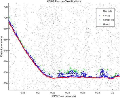
Fig. 4. An example of the classified photons produced from the ATL08 algorithm. Ground photons (red dots) are labeled as all photons falling within a point spread function distance of the estimated ground surface. The top of canopy photons (green dots) are photons that fall within a buffer distance from the upper canopy surface, and the photons that lie between the top of canopy surface and ground surface are labeled as canopy photons (blue dots). (Neuenschwander & Pitts, 2019)
Providing all the potentially useful information from all these processing steps results in a data file that looks like:
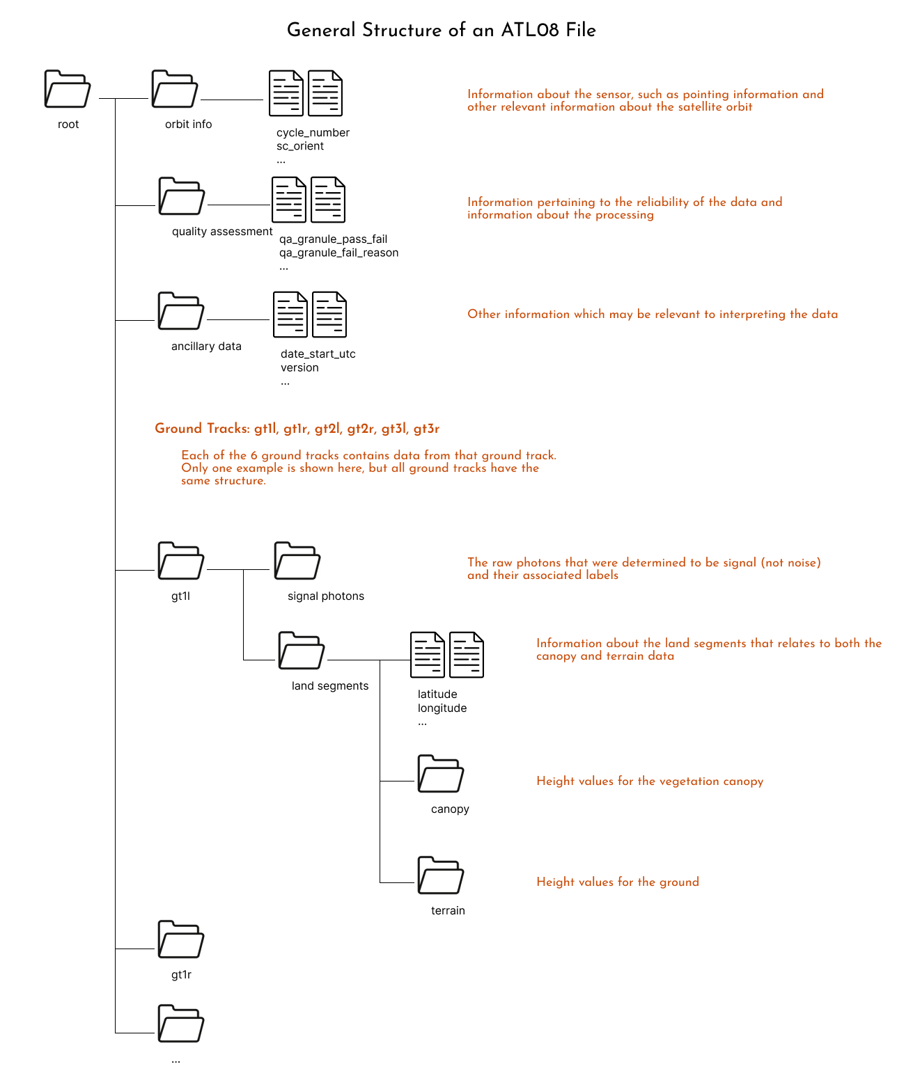
Another way to visualize these structure is to download one file and open it using https://myhdf5.hdfgroup.org/.
Further information about each one of the variables is available in the Algorithm Theoretical Basis Document (ATBD) for ATL08.
There is lots to explore in these variables, but we will move forward using a common ATL08 variable: h_canopy, or the “98% height of all the individual relative canopy heights (height above terrain)” (ATBD definition).
reader.vars.append(var_list=['h_canopy', 'latitude', 'longitude'])
Note that adding variables is a required step before you can load the data.
Load the data!#
ds = reader.load()
ds
<xarray.Dataset> Size: 10kB
Dimensions:              (gran_idx: 1, photon_idx: 211, spot: 2)
Coordinates:
  * gran_idx             (gran_idx) float64 8B 5.54e+04
  * photon_idx           (photon_idx) int64 2kB 0 1 2 3 4 ... 207 208 209 210
  * spot                 (spot) uint8 2B 5 6
    source_file          (gran_idx) <U74 296B './bosque_primavera_ATL08/proce...
    delta_time           (photon_idx) datetime64[ns] 2kB 2019-05-04T12:47:13....
Data variables:
    sc_orient            (gran_idx) int8 1B 0
    cycle_number         (gran_idx) int8 1B 3
    rgt                  (gran_idx, spot, photon_idx) float32 2kB 554.0 ... 5...
    atlas_sdp_gps_epoch  (gran_idx) datetime64[ns] 8B 2018-01-01T00:00:18
    data_start_utc       (gran_idx) datetime64[ns] 8B 2019-05-04T12:46:31.876322
    data_end_utc         (gran_idx) datetime64[ns] 8B 2019-05-04T12:48:54.200826
    latitude             (spot, gran_idx, photon_idx) float32 2kB 20.59 ... 2...
    longitude            (spot, gran_idx, photon_idx) float32 2kB -103.7 ... ...
    gt                   (gran_idx, spot) object 16B 'gt3l' 'gt3r'
    h_canopy             (photon_idx) float32 844B 12.12 4.747 11.83 ... nan nan
Attributes:
    data_product:  ATL08
    Description:   Contains data categorized as land at 100 meter intervals.
data_rate: Data are stored as aggregates of 100 meters.Here we have an xarray Dataset, a common Python data structure for analysis. To visualize the data we can plot it using:
ds.plot.scatter(x="longitude", y="latitude", hue="h_canopy")
<matplotlib.collections.PathCollection at 0x7f0ffad48d10>
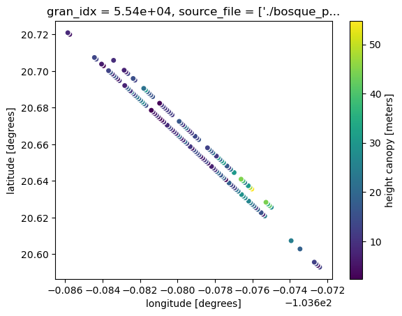
Notice also that the data is shown for just our area of interest! That is because of icepyx’s subsetting feature. You can find more details on this feature in the icepyx example gallery here.
When to Cloud#
The astute user has by now noticed that in this tutorial we downloaded a granule to read in rather than directly reading it from an S3 bucket. Recall from the previous tutorial that reading a single group was a time intensive step and did not include multiple groups. Due to the way ICESat-2 data is stored on disk (because of the file format - it doesn’t matter if it’s a local disk or cloud disk), accessing the data within the file is really slow via the virtual file system. Several efforts are under way to help address this issue, and icepyx will implement them as soon as they are available. Current efforts include:
storing ICESat-2 data in a cloud-optimized format
reading data using the h5coro library
Please let Amy, Jessica, or one of the workshop leads know if you’re interested in joining any of these conversations (or telling us what issues you’ve encountered). We’d love to have your input and use case!
Some example plots#
To close, here are a few more examples of reading and visualizing ATL08 data.
Example 1: View the photon classifications#
# Set up the data reader
reader = ipx.Read('./bosque_primavera_ATL08')
# Add the photon height and classification variables
reader.vars.append(var_list=['ph_h', 'classed_pc_flag', 'latitude', 'longitude'])
ds_photons = reader.load()
ds_photons
<xarray.Dataset> Size: 1MB
Dimensions:              (gran_idx: 1, photon_idx: 25234, spot: 2)
Coordinates:
  * gran_idx             (gran_idx) float64 8B 5.54e+04
  * photon_idx           (photon_idx) int64 202kB 0 1 2 3 ... 25231 25232 25233
  * spot                 (spot) uint8 2B 5 6
    source_file          (gran_idx) <U74 296B './bosque_primavera_ATL08/proce...
    delta_time           (photon_idx) datetime64[ns] 202kB 2019-05-04T12:47:1...
Data variables:
    sc_orient            (gran_idx) int8 1B 0
    cycle_number         (gran_idx) int8 1B 3
    rgt                  (gran_idx, spot, photon_idx) float32 202kB 554.0 ......
    atlas_sdp_gps_epoch  (gran_idx) datetime64[ns] 8B 2018-01-01T00:00:18
    data_start_utc       (gran_idx) datetime64[ns] 8B 2019-05-04T12:46:31.876322
    data_end_utc         (gran_idx) datetime64[ns] 8B 2019-05-04T12:48:54.200826
    latitude             (spot, gran_idx, photon_idx) float32 202kB 20.59 ......
    longitude            (spot, gran_idx, photon_idx) float32 202kB -103.7 .....
    gt                   (gran_idx, spot) <U4 32B 'gt3l' 'gt3r'
    ph_h                 (spot, gran_idx, photon_idx) float32 202kB nan ... 0...
    classed_pc_flag      (spot, gran_idx, photon_idx) float32 202kB nan ... 1.0
Attributes:
data_product: ATL08# Select just one beam. `spot=6` corresponds to the right beam of the 3rd beam pair, gt3r.
gt3r = ds_photons.sel(spot=6)
We can create a simple plot of photon height ph_h above the ground. ATL08 classifies photons as noise, ground, canopy and top of canopy. This classification is accessed through classed_pc_flag. We can use xarray to color photons by type using the hue keyword.
# A less complex plot
fig, ax = plt.subplots()
fig.set_size_inches(15, 4)

gt3r.plot.scatter(ax=ax, x='delta_time', y='ph_h', hue='classed_pc_flag')
<matplotlib.collections.PathCollection at 0x7f0ffac2c510>
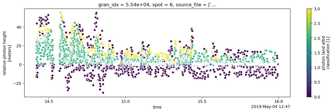
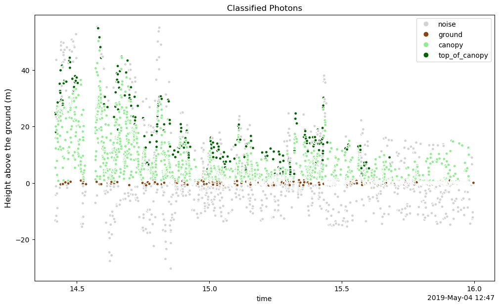
This kind of plot is great for a quick look at the data. A neater plot can also be created by using matplotlib directly to modify the plot above.
We use ListedColormap to create a color map that is more appropriate for vegetation and add a legend, title and y-axis label. The legend labels are read directly from the flag_meanings attribute of the classed_pc_flag variable.
# Created a colormap for classified photons
cmap = ListedColormap(['lightgrey', 'saddlebrown', 'lightgreen', 'darkgreen'])

# Assign flag_meanings to labels to be used in legend
labels = gt3r.classed_pc_flag.attrs["flag_meanings"].split()

fig, ax = plt.subplots(figsize=(12,7))

m = gt3r.plot.scatter(x='delta_time', y='ph_h', hue='classed_pc_flag',
                      s=20,  cmap=cmap,
                      add_legend=False, add_colorbar=False,
                      ax=ax)

handles, old_labels = m.legend_elements()  # Get the legend elements so that labels can be modified
ax.legend(handles, labels)

ax.set_title("Classified Photons")
ax.set_ylabel('Height above the ground (m)', size=12)
Text(0, 0.5, 'Height above the ground (m)')
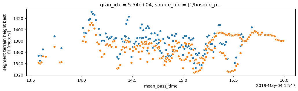
Plot the canopy compared to the ground height#
# Remove our previous variables
reader.vars.remove(all=True)
# Add the next set of variables to the list
reader.vars.append(var_list=['h_te_best_fit', 'latitude', 'longitude'])
# turn off warnings for load to not show an xarray warning that was resolved in the coming release of icepyx v1.0.0
with warnings.catch_warnings(record=True):
    # load the data
    ds_te = reader.load()

ds_te
<xarray.Dataset> Size: 10kB
Dimensions:              (gran_idx: 1, photon_idx: 211, spot: 2)
Coordinates:
  * gran_idx             (gran_idx) float64 8B 5.54e+04
  * photon_idx           (photon_idx) int64 2kB 0 1 2 3 4 ... 207 208 209 210
  * spot                 (spot) uint8 2B 5 6
    source_file          (gran_idx) <U74 296B './bosque_primavera_ATL08/proce...
    delta_time           (photon_idx) datetime64[ns] 2kB 2019-05-04T12:47:13....
Data variables:
    sc_orient            (gran_idx) int8 1B 0
    cycle_number         (gran_idx) int8 1B 3
    rgt                  (gran_idx, spot, photon_idx) float32 2kB 554.0 ... 5...
    atlas_sdp_gps_epoch  (gran_idx) datetime64[ns] 8B 2018-01-01T00:00:18
    data_start_utc       (gran_idx) datetime64[ns] 8B 2019-05-04T12:46:31.876322
    data_end_utc         (gran_idx) datetime64[ns] 8B 2019-05-04T12:48:54.200826
    latitude             (spot, gran_idx, photon_idx) float32 2kB 20.59 ... 2...
    longitude            (spot, gran_idx, photon_idx) float32 2kB -103.7 ... ...
    gt                   (gran_idx, spot) object 16B 'gt3l' 'gt3r'
    h_te_best_fit        (photon_idx) float32 844B 1.342e+03 ... 1.381e+03
Attributes:
    data_product:  ATL08
    Description:   Contains data categorized as land at 100 meter intervals.
data_rate: Data are stored as aggregates of 100 meters.fig, ax = plt.subplots()
fig.set_size_inches(12, 3)
# plot the canopy height above ground level
(ds.h_canopy + ds_te.h_te_best_fit).plot.scatter(ax=ax, x="delta_time", y="h_canopy") # orange
# plot the terrain values
ds_te.plot.scatter(ax=ax, x="delta_time", y="h_te_best_fit") # blue
<matplotlib.collections.PathCollection at 0x7f0ff8b69710>
Summary#
In this notebook we explored the opening and rendering ATL08 data with icepyx. We saw that icepyx will subset our downloaded data to our area of interest and also allows us to download only the variables we need. The ATL08 data has a folder-like structure with many variables to choose from. We focused on h_canopy and showed additional examples using the raw photons and h_te_best_fit for the ground height.
More information about ATL08 or icepyx can be found in:
Neuenschwander et. al. 2019, Remote Sens. Env. DOI