Parallelized Cloud Computing with Dask for Geoscientists

Tutorial by Ellianna Abrahams and Joshua Rines

The following notebook includes materials from notebooks written by Hamed Alemohammad, Ryan Abernathy, Planetary Computer, stackstac, and Dask.

For those that would like to follow along for the introductory section, please install graphviz.

An Introduction to Dask for Parallel Computing¶

Dask is a Python library designed to facilitate parallel computing and distributed data processing. It is particularly useful for handling computations that exceed the available memory of a single machine and for parallelizing tasks across multiple cores or even distributed clusters of machines. The primary goal of Dask is to provide a user-friendly and Pythonic interface for developers to scale their data analysis and processing workflows.

Dask consists of two main components:

1. “Big Data” Collections: Dask provides collections that extend common Python data structures, such as arrays, dataframes, and lists, to handle larger-than-memory or distributed datasets. These collections are designed to mimic the interfaces of popular libraries like NumPy and Pandas, making it easier for developers to transition from single-machine to distributed computing environments.
2. Dynamic Task Scheduling: Dask provides scheduling that manages the distribution and execution of tasks across the available computing resources. It ensures that computations are carried out efficiently in a parallelized manner.

High level collections are used to generate task graphs which can be executed by schedulers on a single machine or a cluster.

Some reasons why you should consider using Dask for your large data:

• Scalable Parallel Computing: Dask enables the parallelization of computations across multiple cores and distributed clusters, allowing users to efficiently handle data processing tasks that exceed the memory capacity of a single machine.
• Lazy Evaluation: Dask adopts a lazy evaluation approach, deferring the execution of operations until explicitly requested. This optimizes the scheduling and execution of computations, enhancing overall efficiency.
• Flexibility Across Data Structures: Dask provides “Big Data” collections that extend common Python data structures (e.g., arrays, dataframes, bags) to handle larger-than-memory or distributed datasets. This flexibility allows users to seamlessly transition between single-machine and distributed computing environments.
• Integration with Distributed Computing: Dask seamlessly integrates with a task scheduler, facilitating the scaling of computations from a single machine to distributed computing clusters. This adaptability makes Dask a versatile tool for handling diverse big data processing scenarios.

In essence, Dask offers a versatile and user-friendly framework for scalable, parallel, and distributed computing in Python, making it well-suited for a wide range of data analysis and processing tasks.

Dask Arrays¶

Today, we’ll be focusing on processing image data, i.e. array data, with dask, but it can also be used with most any familiar python data variables, like dataframes (pandas-like) for example.

A dask array is very similar to a numpy or xarray array. However, a dask array is only symbolic, and doesn’t initially hold any data. It is structured to represent the shape, chunks, and computations needed to generate the data. Dask remains efficient by delaying computations until the full computation thread is built up and the data is requested. This mode of operation is called “lazy evaluation” and this mode allows users to build up a symbolic thread of calculations before turning them over the scheduler for execution.

dask arrays arrange many python arrays into a grid. The underlying arrays are stored either locally, or on a remote machine like the cloud.

Let’s compare some numpy arrays to dask arrays to illustrate further how Dask operates. We’ll begin by creating a numpy array of ones.

Let’s look at the size of this array in memory:

Now, we’ll create the same array in dask.

Notice how this array comes with a dask visualization of our array and includes the word “chunks.” Chunks are the way that dask splits the array into sub-arrays. We did not specify how we wanted to chunk the array, so dask just used one chunk for the whole array. At this point, the dask array is very similar to the numpy array and isn’t structured to take advantage of dask functionality.

Specifying Chunks¶

To leverage the full power of dask, we’ll split our array into specified chunks. The Dask documentation provides several ways to specify chunks. In this demonstration, we’ll use a block shape.

At this point, all we have is a symbolic represetnation of the array, including its shape, data type, and chunk size. This is an example of lazy evalution; unlike numpy, dask has not generated data yet.

In order to generate data, we need to send the data collection to the scheduler, which we can do by calling the compute function.

Dask has a nifty visualize function that illustrates the symbolic operations that ran when we called compute.

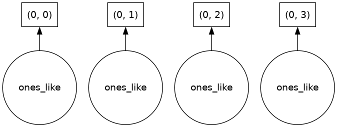
We can see that we stored four “ones-like” arrays, one in each chunk. To generate the data, the dask scheduler calls np.ones four times and then concatenates all of them together into one array.

Rather than immediately loading a dask array (which will store all of the data in RAM), we usually would like to do some kind of analysis on the data and don’t necessarily want to store the full raw data in memory. Let’s see how dask handles a more complex computation that reduces the data.

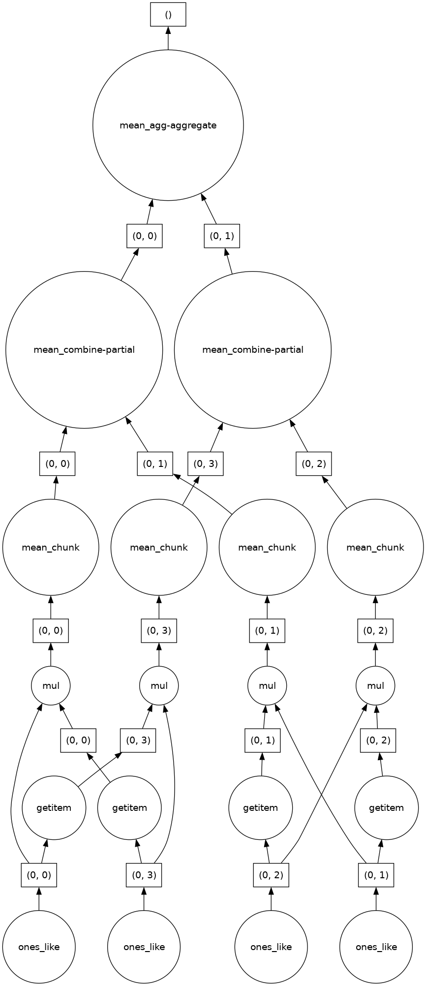
We can see Dask’s strategy for running the calculation thread on our data array. The power of Dask is that it automatically designs an algorithm appropriate for complex operation threads with big data.

Monitor Dask Usage via Dask Dashboard¶

Dask offers visualization tools for you to monitor how dask is using memory across your cluster of CPUs and GPUs. This is important when working with large data, because as we’ll see later in this tutorial certain computations can actually add memory usage, potentially exceeding your memory amount while a task is being run or doubling up on computation time making them better to complete outside of dask.

Let’s take a quick look at the dask dashboard which is available to us in CryoCloud.

On the left of our screen we’re going to open the dask dashboard. We’ll copy the path listed above in the client into the dashboard to connect our CryoCloud instance to a dashboard. Once the dashboard is up and running, please click on “Task Stream,” “Progress,” “Workers Memory,” and “Graph.”

For the sake of time today, we’ll just look at a couple of the assessment tools available to us in the dask dashboard, but the dask documentation with a more extensive list on what diagnostics are available to you through the dashboard.

Dask For Geoscientific Images¶

For this section of the tutorial, we’re going to move into using dask with data types that are of interest to us in the Cryosphere. We’ll work with Landsat data and use dask’s native functionality to stream this data in directly from the cloud while only bringing in the pixels that we are interested in. Once we’ve selected our data of interest, we’ll use machine learning tools that interact with dask to do a basic image segmentation task.

Learning Goals:¶

• Interacting with a Large Image using Dask
  • Query a Landsat time-series using stackstac with Planetary Computer
  • Refine the image query before downloading data
  • Import the refined image
• Running Custom Functions on Dask + xarray
  • Using a custom function for analysis before importing data
  • Implementing scikit image on dask arrays
• Generating a Deep Learning Dataset using sat-tile-stack
  • Importing time-series imagery into a tiled, machine learning-ready, Dask-enabled format
  • Appending spatial masks to emphasize relavent areas in the image tiles
  • Appending metadata for cloud metrics and tile completeness (e.g., track which tiles in the time-series are usable)

Computing Environment¶

We will set up our computing environment with package imports. Today we’ll be working with planetary computer, dask, xarray, and scikit image.

Tip: If you need to import a library that is not pre-installed, use pip install <package-name> in a Jupyter notebook cell alone to install it for this instance of CryoCloud. On CryoCloud, your package installation will not persist between logins.

Interacting with a Large Image Using Dask¶

Data Import using Planetary Computer and Stackstac¶

The Planetary Computer package allows users to stream data stored in Microsoft’s Planetary Computer Catalog directly from the cloud. When combined with stackstac tools, this allows users to query an area of interest and planetary computer will stream all the requested data from that area using dask.

In this tutorial, we are using Planetary Computer to interact with images from Landsat. In particular, we’ll query images that are around the San Francisco Bay, where this tutorial is taking place. To initialize planetary computer, we’ll define a catalog variable and define the coordinate bounds of our image query using rasterio.

Now we’ll define a time range to search over and the Landsat bands that we are interested in. In our query we limit the data to images that have cloud cover (eo:cloud_cover) less than (lt) 20%.

Notice how items has created a pystac item collection of all the relevant image slices from Landsat that are located within our coordinate bounds. Now we’ll use stackstac to turn these into a Dask xarray that we can interact with.

That was fast for a large image cutout! Let’s figure out why. Take a look at the bottom of your CryoCloud Screen and check your memory. You’ll notice that it should be on the order of MBs at this point, and this is because we haven’t yet pulled any data into our CryoCloud environment. Instead we have the directions to the data locations for all of the Landsat images in Planetary Computer, ready to stream into an initialized xarray.

Under the hood, stackstac is using dask to do this. Currently we have the “lazy” load we discussed above implemented. dask allows you to perform parallel and distributed computing on larger-than-memory datasets, but this can be inefficient. Lazy evaluation delays the execution of operations, here that would be pulling in the data to your CryoCloud instance, until the results are actually needed. This approach enables dask to efficiently handle large computations. What we see in the printout above is a symbolic representation of the xarray dimensions for our data.

Why is this evaluation using any memory at all? Check above and see that the table describing your xarray has a row named “Dask Graph.” There we see that our data would be divided into chunks and graph layers. As part of the lazy load, dask has initialized these chunks as empty variables and that is what is currently using memory.

How big would this dataset be if we held it all in memory?

Refining our Image Before Data Import¶

We know that we have a time-series of 696 images, but perhaps we’re actually interested in behavior averaged over monthly timescales in this region and we only want an rgb image. We can manipulate our stackstac array just like we would with a regular xarray.

Notice how we got a warning that dask is automatically adjusting the chunk size for our xarray object. In dask, the chunk size is a critical parameter that determines how the data is divided into smaller, manageable pieces for distributed processing. When you create or manipulate a dask enabled xarray dataset, dask tries to find an appropriate chunk size based on the size of the data and the available computing resources. This adjustment is made to optimize computational performance once we finally compute our evaluation. For now, we are still in a lazy state, which you can see evidenced by how little memory we are taking up.

We have queried for a rather large image size, and if we were to pull all of that down to our local machine, we might overwhelm the amount of memory available to us on our current CryoCloud instance. Luckily, we can keep using our dask-enabled xarray to further refine our query before pulling the data in. Let’s reproject our data to UTM coordinates so we can pick a specific area of interest based on a length of distance in the x/y plane.

Import the Refined Image¶

Now that we’ve refined our query, without overloading the memory, we can import the refined time-series. This will allow us to do further calculations with it on our CryoCloud instance, or even just allow us to visualize it. Let’s see what we’ve been working with!

Even though we visualized pathways for our toy array above using the built-in visualize function, we don’t recommend running it here, as this will take too long to load.

The compute function in dask triggers the actual data pull. We can monitor the time that it takes using the dask progress bar. While this is processing watch the memory at the bottom of the screen.

Notice how the memory fluctuated, and at times was much higher than the final memory. dask still needed to bring all the data into our cloud instance, but only needed to hold the data from our initial query in memory as long as it was needed to do our calculations. We are now left with a much smaller slice than our initial query, but the slice that we wanted, which a monthly-averaged Landsat time series of a specific area on the map. Now that the data that we wanted all along is in our CryoCloud RAM, let’s visualize it.

First we’ll take a look at data. It’s still an xarray, but we can see that the data is present, and it is no longer held in chunks. Since we know that Landsat doesn’t pass over this location every month, we’ll eliminate the time slices that have no data in them.

We’ll use xarray’s native plotting function to visualize the data.

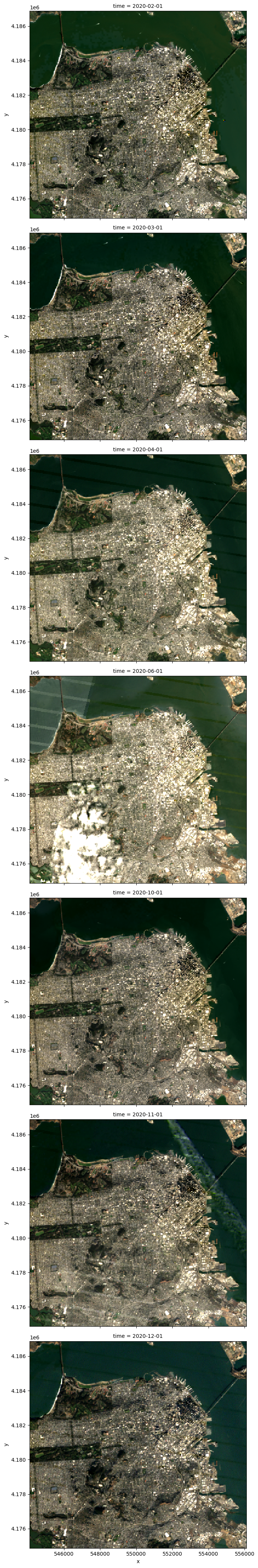
Running Complex Python Functions with Dask + Xarray¶

In the previous section we showed how dask can be used to pull data from the cloud while refining your search ahead of time to the data and resolutions that you are interested in. In this section we’ll see how dask can be used to do some more complex analyses as well before pulling the data into memory.

dask does have a native package for interacting with images called dask_image, but it can be tricky to use with streaming data in chunks, which makes it difficult to use on large images stored elsewhere in the cloud. We will instead write some custom functions to be used on our dask data, so that we can import our data already transformed.

Implementing Custom Functions with Dask¶

Let’s start by looking at the normalized difference vegetation index (NDVI). In the cryosphere, this isn’t likely to be an index that we use often, but it’s a great stand in for how we can create custom functions in dask. This same principal could be applied to pull in our data as band ratios, or other preprocessing functions that we might be interested in. Similarly to above, we’ll limit this to our area of interest.

Perhaps we are also interested in obtaining an average NDVI across the entire year. Like before we can write this calculation before computing so that we only keep the data that we’re interested persistant in memory. The persist function is an alternative to calling compute that triggers the computation and stores the results so that subsequent computations can reuse these stored values. This can be useful if we intend to repeat a calculation.

We can visualize this using dask’s built in plotting functionality.

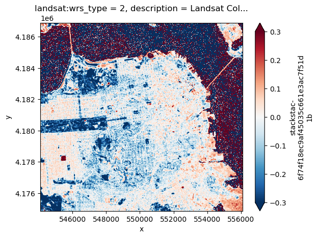
Operating Sci-kit Image with Dask for Quick Segmentation¶

What if we want to do something more complicated, like something that requires packages from sklearn? We can also pair sklearn functionality with dask arrays. First we’ll take the yearly average of the luminance of our data.

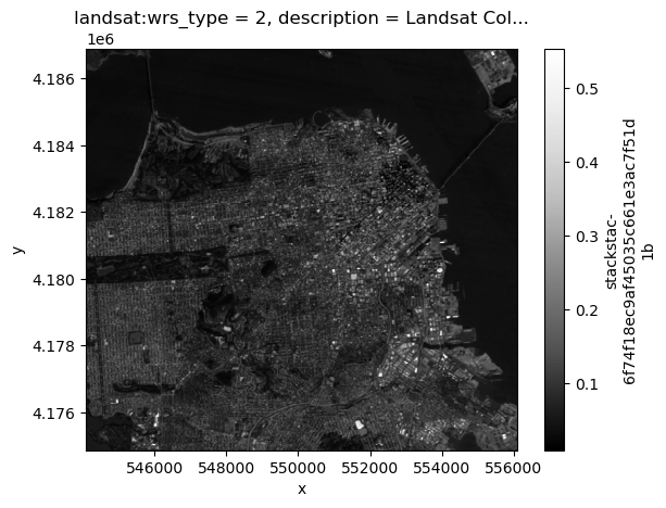
We still haven’t computed our data, so this is still operating in lazy load, which means that even though we had to bring the data into memory for our plot we didn’t hold it there, and so dask produced the image and then removed the data from memory.

We are about to switch over to using a function from another package, sci-kit image, and this function will require pulling the data into memory in order to run a more complex function. This means that it is important to have enough memory to allow for the function to store whatever copies of the data it needs while it is computing, but it will only save the output in memory.

Once we have run a gaussian filter on our data, we can run a simple threshold our images for a basic segmentation. This will not be as nice as segmentation done with more complex computer vision methods, but can be useful for finding easily delineated objects.

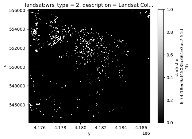
If we wanted to run machine learning models using sci-kit learn we could apply the same principle. The really beautiful thing about using dask for these tasks is that our initial dataset was estimated to be >600 GB, and we are able to do these relatively high level tasks while streaming in only 20.22 GB that we needed. If we needed to be careful, we could be even more specific about how we implement dask to ensure that we are incredibly efficient with our persistant memory usage.

For a deeper dive into using dask with an applied Cryosphere project, head to Jonny Kingslake’s tutorial on using ARCO data with zarr and dask.

Generating a deep learning-ready dataset from satellite imagery¶

Let’s say you’re now interested in training a deep learning model to automatically detect changes that are happening in a region over time. For example, suppose you are curious about tracking container ships that visit two of the Oakland Seaport ports over time. Temporal deep learning models typically require consistent tile sizes, such as 256x256 pixels, as well as a consistent time step cadence, such as daily. We can take advantage of a convenient function, sat-tile-stack, built on dask and stackstac to compile a stack of imagery across time that is ready for use in training a deep learning model.

Install sat-tile-stack¶

Let’s install sat-tile-stack from github, which will allow us to quickly compile a stack of tiled satellite imagery across time at a daily cadence. Don’t worry if you see an ERROR: pip's dependency resolver does not... pop up, the install still worked.

Import depencencies¶

Next, we will import all the relevant dependencies (many of these are repeated from earlier parts of this tutorial, but we will re-import them nonetheless).

Generate a tilestack¶

We can now call sattile_stack to generate our tile stack, which will come in as a DataArray. Note here that we have the option to generate a mask band which will be appended to the DataArray. In our example, let’s say we wanted the flexibility to test out an attention layer in our deep learning network which would focus the learning on the shipping dock terminals. This mask is a .geojson file, to which we simply grant the function sattile_stack access, and a mask will be appended to the end of the band coordinate in our DataArray. To access the mask for this example, please go to https://github.com/CryoInTheCloud/CryoCloudWebsite/tree/main/book/tutorials and find the oakland_port_terminals.geojson file. Place the file in the same directory out of which you are operating this tutorial. Ensure the file path to this mask file is correct in the line filepath_mask = "/path/to/oakland_port_terminals.geojson".

Let’s take a look at our tilestack:

Analyze cloudy days and no-data days¶

As we will see, some days we have relatively useless imagery. This can be for one of two main reasons: (1) clouds or (2) no image acquisition. The satellite constellation that we are using here, Sentinel 2, has a repeat cycle of ~5 days, giving us an image of the same spot on Earth every 5 days. Despite the fact that we need to maintain a regular cadence (e.g., daily) for feeding our deep learning model, we might also want to keep track of whether or not a particular image is useful, which can be a sort of metadata we can feed to the model to help guide the learning. To do this, we can make a calculation based on whether any given tile is (1) too cloudy or (2) contains too many nans to be useful (e.g., no imagery acquired on that day). We show how do this below, extracting these percentages directly from our tilestack.

From our tiles in tilestack, we can build a dataframe using Pandas (pd) to look at the cloud cover and percentage of NaNs for each tile along the time dimension.

And we can look at what that dataframe is by calling it. The first column is the date, second colum is the cloud cover percentage, third column is the NaN percentage. You’ll notice later in the tutorial when we plot these tiles that the cloudiness percentage doesn’t necessarily line up with how many clouds we can visually see. This is because the cloudiness percentage is calculated on a larger spatial scale. The tiles we generate are effectively ‘cut out’ from larger image strips that are acquired by the satellites. The cloudiness is computed at the scale of these larger image strips, so it could be the case that there is a higher percentage of clouds somewhere in the larger strip, but not directly over where we chose to cut the tile. That being said, this is still a good first order step in integrating cloudiness metadata into our datasets and later into a machine learning model.

Plotting¶

Below we write a few quick helper functions to visualize the time-stacked tiles. The first function is a linear stretch, which remaps the pixel values of the tiles so to enhance contrast by discarding extreme values. The second function will display the tiles in our stack starting on the date you chose and extending for ndays. The plot will put the tiles into an array with ncols columns.

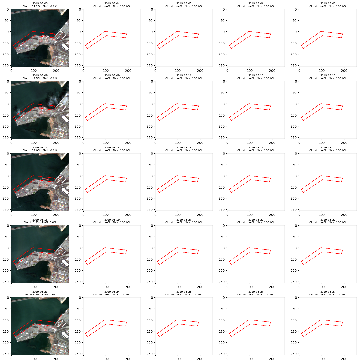
We can see in the above example that there are two ports at this location, one extending horizontally and one more diagonally. If you look closely you can see ships coming and going from both of these ports. This is the sort of task that we might want to automate with a machine learning algorithm. This stack of tiles can now be used in a deep learning model, and is readily adaptable for requirements such as cloud cover, nan-thresholds, and mask-based spatial attention.